Denormalization Depth Decisions for Analyst-Facing Tables

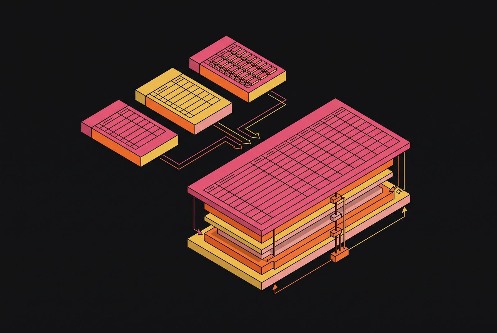
Transactional systems and analytical systems are built to do different jobs, and the schemas that serve them inherit that split. A schema tuned for the first job penalizes the second, and a schema tuned for the second would be reckless for the first.

It prevents update anomalies, the situation where the same fact lives in multiple rows and an update to one copy leaves the others wrong, and that protection matters in a system processing constant writes. It matters far less in a system that mostly reads, and the cost of keeping that protection in place grows the moment the workload shifts: every join needed to reassemble a normalized record adds latency, adds complexity to the query plan, and adds a barrier for anyone trying to write ad hoc SQL without a data engineering background.

Cloud columnar engines change the storage math that used to justify normalization on cost grounds alone. Redundant string values compress aggressively in a columnar store, so a denormalized table carrying a repeated customer name or region label across a billion rows does not carry anywhere near a billion times the storage cost of a single unique value. The gap in storage footprint between a normalized and a denormalized version of the same data is often small enough not to factor meaningfully into the decision.

None of this means an analytical table should be built from scratch without any normalization discipline behind it. A properly built analytical layer takes an already-normalized upstream source and deliberately flattens it during the load process, with the canonical, normalized version still sitting upstream as the source of truth. The denormalized table is a derived, rebuildable artifact, not a replacement for discipline further back in the pipeline. That distinction sets up the real question this piece is built around: not whether to denormalize, but at which layer of the warehouse that flattening should happen, and how far it should go.

How warehouse layers determine which normalization rules apply where

Each layer of a modern warehouse answers normalization differently, so the design task is to locate the right boundary between normalized and denormalized schemas for that layer. Thinking of the warehouse in rough stages, source and staging, a core or integration layer, a mart or analytical layer, and a reporting or wide-table layer, makes the boundary easier to place, in the same spirit as the tiered staging common to lakehouse architectures, without needing to adopt that platform model wholesale.

The mart or analytical layer is where denormalization becomes the default. This is the layer analysts query directly, the layer BI tools connect to, and increasingly the layer AI agents query as well, so it should be shaped around reads.

The reporting or wide-table layer pushes that same logic further, favoring pre-aggregated rollups and one-big-table patterns wherever the questions being asked are stable and well understood in advance. The decision a team actually faces is where the boundary between normalized and denormalized schemas should sit, and that boundary depends on how often the underlying data changes, how stable the schema is, who or what is consuming it, and what the queries against it actually look like.

Star schema as the practical middle ground

Star schema earns its place as the default analytical pattern because it commits to a specific, bounded depth: one join between a fact table and its surrounding dimension tables, never more. Modern engines like Snowflake, BigQuery, Redshift RA3 and serverless, and Databricks SQL handle four-join and five-join query plans without strain, which is part of why star schema's modest join depth barely registers as a performance cost.

The structure itself is simple: a central fact table carries measures and foreign keys, dimension tables around it carry descriptive attributes, and queries reach outward exactly one hop to pull in whatever context they need.

Dimension updates make the strongest case for keeping that one hop in place. Normalization's update-anomaly protection, which matters so little in a pure read workload, earns its keep here precisely because dimensions change even when facts don't.

Slowly changing dimensions, specifically Type 2 SCDs, make the case even more concretely. A fully flattened one-big-table design has to replicate that same accuracy by embedding historical snapshot attributes directly into every fact row, which is a far costlier way to get the same guarantee.

Star schema also holds its position because it stays legible to the humans using it. A 150-column OBT carrying embedded historical dimension snapshots needs documentation just to be queried safely, and that documentation burden is itself a cost of depth, not just a cost of performance.

The snowflake schema takes the opposite direction from OBT: it normalizes dimension tables further into sub-dimension tables, preserving more of normalization's update efficiency at the cost of additional join depth. That trade-off makes sense when dimension hierarchies are large, change frequently, and get shared across multiple fact tables, but it gives up the query simplicity that makes star schema the default choice for most analytical layers. Star schema's one join is already a commitment, not a given, and the sections that follow argue for both directions away from it: going flatter under specific conditions, and staying partly normalized under others.

Small lookup tables and the case for partial snowflaking within an otherwise flat layer

Committing to denormalization at the mart layer does not mean every dimension should be embedded into every fact table that touches it. Small, stable, widely shared lookup tables are the clearest exception, and they often belong in their own normalized table even inside an otherwise flat schema.

Embedding a table like that into every fact table that references it produces many redundant copies of data that essentially never changes and was never expensive to join.

The cost-benefit math here runs in the opposite direction from the usual denormalization argument.

Deciding exactly which dimension hierarchies qualify for this treatment and which should be fully embedded is a judgment call. The rough line runs along dimension size, how often the dimension updates, and how widely it's shared across fact tables, and reasonable teams will draw that line in slightly different places depending on their own pipelines.

Partial snowflaking, keeping a handful of dimension hierarchies normalized inside an otherwise mostly-flat schema, is a legitimate middle position. Its risk is inconsistency: join depth that varies table to table makes the schema harder to document in full and makes self-service query writing less predictable for analysts who learned the schema from one table and assumed the pattern held everywhere.

Conditions that justify one-big-table

One-big-table is not a shortcut taken under deadline pressure or a sign of a design that gave up partway through.

OBT collapses every join to zero at query time by doing that join work once, at build time, instead. The payoff is that query performance scales with row count alone rather than with join complexity, a predictability that even a shallow star schema cannot fully match, because a star schema's query plan still depends on how the optimizer handles the join.

A handful of conditions tend to justify reaching for OBT specifically. Self-service BI environments, where business users pick fields from a flat table through a drag-and-drop interface rather than writing SQL, are one: these users cannot and should not be expected to understand multi-table join logic, so the table has to arrive pre-joined. AI-generated SQL is a second, and a fast-growing one: when an AI agent is the one writing the query, fewer tables and fewer possible join paths directly reduce the chance that the agent picks a wrong join condition or invents a relationship that doesn't exist in the schema. OBT only pays for its own construction cost when the questions it answers are durable enough to justify that investment. Machine learning feature stores round out the list: training and inference pipelines need wide, row-level, historically complete tables, and the wide format of OBT maps directly onto the feature matrix those pipelines consume.

The costs that come with those benefits have to be accepted deliberately. Schema rigidity is the sharpest one: adding a new dimension to an existing OBT means a pipeline change, a schema change, and potentially a full backfill, where the same addition to a star schema is just a new dimension table and a foreign key.

Many production architectures run both at once, maintaining star schemas in the mart layer for general analytical use while building OBTs on top of them for specific reporting surfaces or specific ML pipelines, each structure serving a different consumer from a different physical table.

How query access patterns should drive the depth decision

The right depth for any given table comes from analyzing who queries it, how they query it, and how often its underlying dimensions change, not from whichever schema convention a team happens to have learned first.

A short set of questions does most of the work of that analysis. If query latency is already acceptable at the current join depth, adding denormalization solves a problem that doesn't exist yet and introduces maintenance cost for no return. If the source dimension data changes frequently and any staleness in that data is unacceptable, the update cost that comes with a deeply denormalized table can outweigh whatever query speed it buys, and a materialized view becomes the better middle path: it pre-joins the data without committing to full physical flattening everywhere downstream. If the consumer is a BI tool, a self-service analyst, or an AI agent writing its own SQL, flatter is the safer choice; if the consumer is an experienced analyst comfortable with complex queries, or a data engineer building further transformations on top, the join depth of a star schema or even a snowflake schema is perfectly manageable.

Pre-aggregated rollup tables, daily or monthly summaries built on top of a more granular denormalized base, extend this same logic one step further: they trade away row-level granularity for faster reads, and that trade only makes sense when the dashboard consuming them always queries at a fixed grain and never needs to drop down to row-level detail.

Materialized views sit in a specific spot in this framework. They give a query the simplicity of a wide flat table while keeping the redundancy physical rather than computed live, because the underlying join runs once at creation or refresh time and the result is stored on disk. That makes them the right tool when live-join latency is unacceptable but the rebuild cost of a full OBT is unacceptable too.

Access pattern analysis frequently reveals a conflict that no single schema can resolve. In that situation, the access pattern analysis itself is the evidence that two separate physical schemas are the correct answer, not a sign that the modeling was done wrong the first time.

Security, Compliance, and Data Exposure at the Analytical Layer

How far a schema gets flattened determines how widely sensitive fields end up distributed across it, and that distribution directly sets the blast radius of any access misconfiguration along with the complexity of enforcing controls over it.

In a normalized schema, PII fields such as email addresses, national identifiers, and payment details stay isolated in a single table governed by a single access control policy. In a deeply denormalized wide table, those same fields get copied onto every fact row, sitting alongside operational metrics, so every role with access to the fact table now has a path to the PII as well, whether or not that was the intent.

Dynamic data masking offers a way to protect those fields while preserving access to the table: analysts see masked values for any field outside their role's permission scope.

For any product that syncs data into a customer's own warehouse or embeds analytics capability directly into its application, the shape of the exported schema carries consequences beyond the vendor's own environment. A deeply denormalized export that places PII next to operational data widens the exposure inside the customer's infrastructure, not just inside the vendor's.

Private-cloud and data residency requirements add one more constraint on top. In environments where data cannot cross a defined regional or infrastructure boundary, the schema design of analytical tables has to be compatible with however the pipeline that builds and maintains them is deployed, and a pipeline that depends on a managed cloud hop to rebuild a denormalized table may simply be incompatible with a strict residency rule, regardless of how well that schema performs on query speed alone.

How AI agent access raises the stakes on schema clarity and depth decisions

AI agents querying a warehouse directly turn a poor schema depth decision into a much costlier mistake than it would be with a human analyst at the keyboard. A deeply normalized schema with cryptic table names forces an agent to infer join paths on its own, and a wrong inference produces wrong SQL, which produces wrong answers delivered at whatever scale the agent is operating.

Denormalization addresses that problem directly. A flat or near-flat table with descriptive column names gives an agent a single surface to reason about, cuts the number of join decisions it has to make down to zero or close to it, and makes the meaning of each column legible from its name alone rather than from documentation the agent may never see.

Role-based access control applied at the schema level is the necessary complement to that clarity. Restricting which tables, columns, and roles an agent can reach keeps the internal normalized schema from being exposed directly to an external or automated consumer, while still letting a clean, denormalized surface be queried safely on top of it.

Teams building products where AI agents access synced or exported data face this decision at the product layer, not only inside their own internal warehouse. The schema shape of whatever surface is exposed to those agents, whether through an API, an MCP server, or direct warehouse access, sets the accuracy floor for every AI-driven feature built on top of it.